Temporal Feature Alignment and Mutual Information Maximization for Video Based Human Pose Estimation
review one of the applications of the information bottleneck method.
Multi-frame human pose estimation is one of very interesting problem in computer vision. Accurate estimation in the problem is disturbed by ambiguous images due to fast movement, intersections or blockings of objects. There are at least 3 method in this domain: image-based estimation, video-based estimation and feature alignment. In the paper, the authors used the feature alignment method which supplements the key frame feature by extracting coarse-to-fine ones from the neighbor frames. Furthermore, they applied mutual information (MI) to maximize the task-relevant information.
Main
- Notation
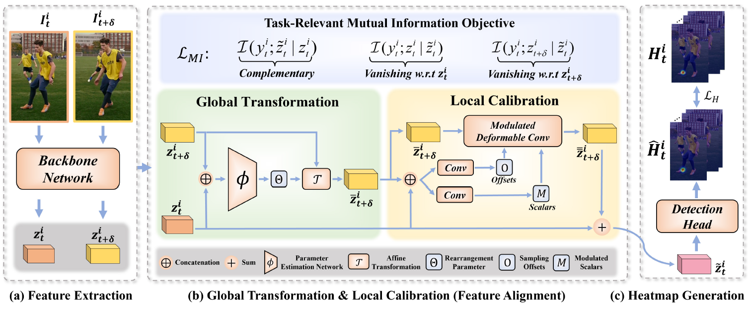
– \(I_t^i\): the cropped video frame of a specific person \(i\) at time \(t\)
– \(\{I_{t+\delta}^i \vert \delta \in \mathbb{N}\}\): the supporting (neighboring) frames of \(I_t^i\)
– \(z_t^i\): the feature of \(I_t^i\) extracted from the backbone network
– \(\tilde{z}_t^i\): the enhanced version of \(z_t^i\) by the main model
- The backbone network: HRNet-W48
 figure 1: Overall pipeline of the paper (FAMI-Pose).
1. MI loss
The authors employed the Variational Self-Distillation to optimize the Information Bottleneck. If you are interested in this topic, refer to my review: Farewell to Mutual Information (2021)
First, we need to maximize the information between \(y_t^i\) and \(\tilde{z}_t^i\), complementary to \(z_t^i\).
- sub-opt. 1: \(\max I(y_t^i;\tilde{z}_t^i \vert z_t^i)\)
\(I(y_t^i;\tilde{z}_t^i \vert z_t^i)\) is decomposed into the 3 factors. \[\begin{aligned} I(y_t^i;\tilde{z}_t^i \vert z_t^i) = I(y_t^i;\tilde{z}_t^i) - I(\tilde{z}_t^i;z_t^i) - I(\tilde{z}_t^i;z_t^i \vert y_t^i). \end{aligned}\]
– \(I(y_t^i;\tilde{z}_t^i)\) is the information in \(\tilde{z}_t^i\) relevant to \(y_t\).
– \(I(\tilde{z}_t^i;z_t^i)\) is the information shared by \(\tilde{z}_t^i\) and \(z_t^i\).
– \(I(\tilde{z}_t^i;z_t^i \vert y_t^i)\) is the information contained in \(\tilde{z}_t^i\) which is dependent to \(z_t^i\), but irrelevant to \(y_t^i\).
The authors argues that we can ignore the irrelevant information, \(I(\tilde{z}_t^i;z_t^i \vert y_t^i)\), during the training, since the relevant information overwhelms the irrelevant one heuristically. Therefore we use the following approximation: \[\begin{aligned} I(y_t^i;\tilde{z}_t^i \vert z_t^i) \approx I(y_t^i;\tilde{z}_t^i) - I(\tilde{z}_t^i;z_t^i). \end{aligned}\]
Next, we have to minimize MI \(I(y_t^i;z_t^i)\) and \(I(y_t^i;z_t^{t+\delta})\), complementary to \(\tilde{z}_t^i\).
- sub-opt. 2. \(\min \{ I(y_t^i;z_{t+\delta}^i \vert \tilde{z}_t^i) + I(y_t^i;z_t^i \vert \tilde{z}_t^i) \}\)
Similarly, we use the following approximations: \[\begin{gathered} I(y_t^i;z_{t+\delta}^i \vert \tilde{z}_t^i) \approx I(y_t^i;z_t^{t+\delta}) - I(z_{t+\delta}^i;\tilde{z}_t^i), \newline I(y_t^i;z_t^i \vert \tilde{z}_t^i) \approx I(y_t^i;z_t^i) - I(z_t^i;\tilde{z}_t^i). \end{gathered}\]
By combining these approximations, we can optimize not only the complementary information term but also the 2 regularization terms as follows: \[\begin{aligned} \mathcal{L}_{MI} = -\lambda \cdot I(y_t^i;\tilde{z}_t^i \vert z_t^i) + I(y_t^i;z_{t+\delta}^i \vert \tilde{z}_t^i) + I(y_t^i;z_t^i \vert \tilde{z}_t^i) \end{aligned}\]
with the coefficient \(\lambda\).
2. MI loss estimation in python
The authors also provide their code here.
Let us look into the python code.

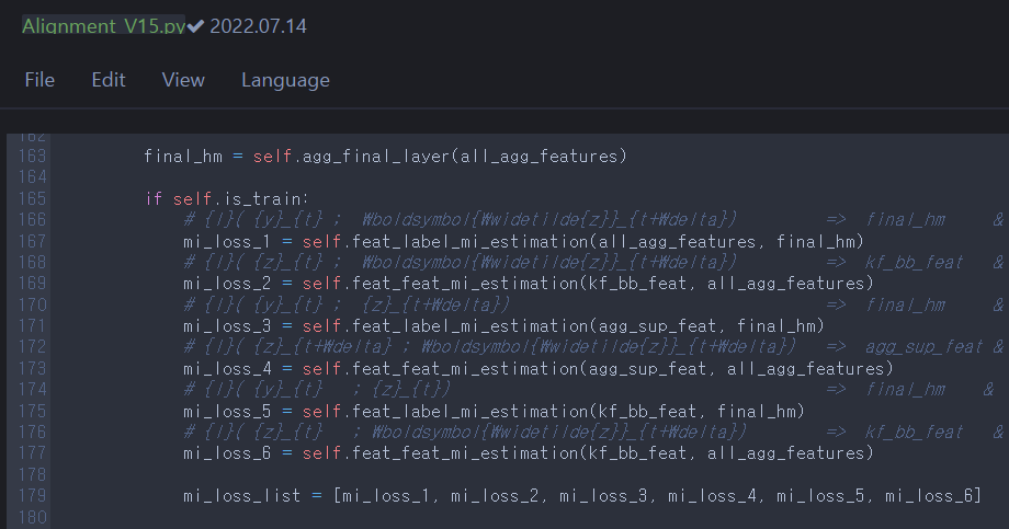
Each MI_loss_i corresponds to the following equations like:
MI_loss_1 = \(I(y_t^i;\tilde{z}_t^i)\)
MI_loss_2 = \(I(\tilde{z}_t^i;z_t^i)\)
MI_loss_3 = \(I(y_t^i;z_t^{t+\delta})\)
MI_loss_4 = \(I(z_{t+\delta}^i;\tilde{z}_t^i)\)
MI_loss_5 = \(I(y_t^i;z_t^i)\)
MI_loss_6 = \(I(z_t^i;\tilde{z}_t^i)\)
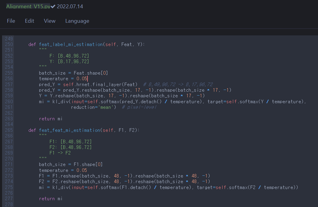
Then let us figure out what ‘feat_label_mi_estimation’ and ‘feat_feat_mi_estimation’ are.

Excluding other techniques, they are torch.nn.functional.kl_div; i.e., they are just Kullback-Leibler divergence (relative entropy).
However, KL divergence and MI are related but distinct to each other.
How is this possible?
The solution is, in my opinion, as follows:
Through the invertible transformation \(D\) (detection head), we estimate \(y\) from \(\tilde{z}\); i.e, \(\hat{y}=D(\tilde{z})\). Thus \(\hat{y}\) has the estimated distribution \(p(\hat{y}) = q(y)\). For independent and identically distributed \(Y_1\) and \(Y_2\), \[\begin{aligned} I(y;\tilde{z}) &= I(y;\hat{y}) \newline &= KL(p(y_1,y_2) \parallel p(y_1)q(y_2)) \newline &= -\sum_{y_1}\sum_{y_2}p(y_1,y_2)\log\frac{p(y_1)q(y_2)}{p(y_1,y_2)} \newline &= -\sum_{y_1}\sum_{y_2}p(y_1)p(y_2)\log\frac{p(y_1)q(y_2)}{p(y_1)p(y_2)} \newline &= -\sum_{y_1}p(y_1)\sum_{y_2}p(y_2)\log\frac{q(y_2)}{p(y_2)} \newline &= -\sum_{y}p(y)\log\frac{q(y)}{p(y)} \newline &= KL(p(y) \parallel q(y)) \newline &= KL(p(y) \parallel p(\tilde{z})). \end{aligned}\]
Reference
- Liu, Zhenguang, et al. “Temporal feature alignment and mutual information maximization for video-based human pose estimation.” Proceedings of the IEEE/CVF conference on computer vision and pattern recognition. 2022.
