Attention is All You Need
review the paper of the transformer.
In the sequence data domain, ML models based on recurrent or convolutional neural networks were dominant. However, even though many improvements have been made to them, there exist intrinsic limitations in the RNN and CNN. In 2017, the authors released the transformer that uses only the attention mechanism and no recurrence or convolutions at all, which is currently the most common technique in the field.
1. Model Architecture
The transformer [1] is an auto-regressive model with encoder-decoder structure. An auto-regressive model of order \(p\) can be written as \[y_t = c + \phi_{1}y_{t-1} + \phi_{2}y_{t-2} + \dots + \phi_{p}y_{t-p} + \epsilon_t\]
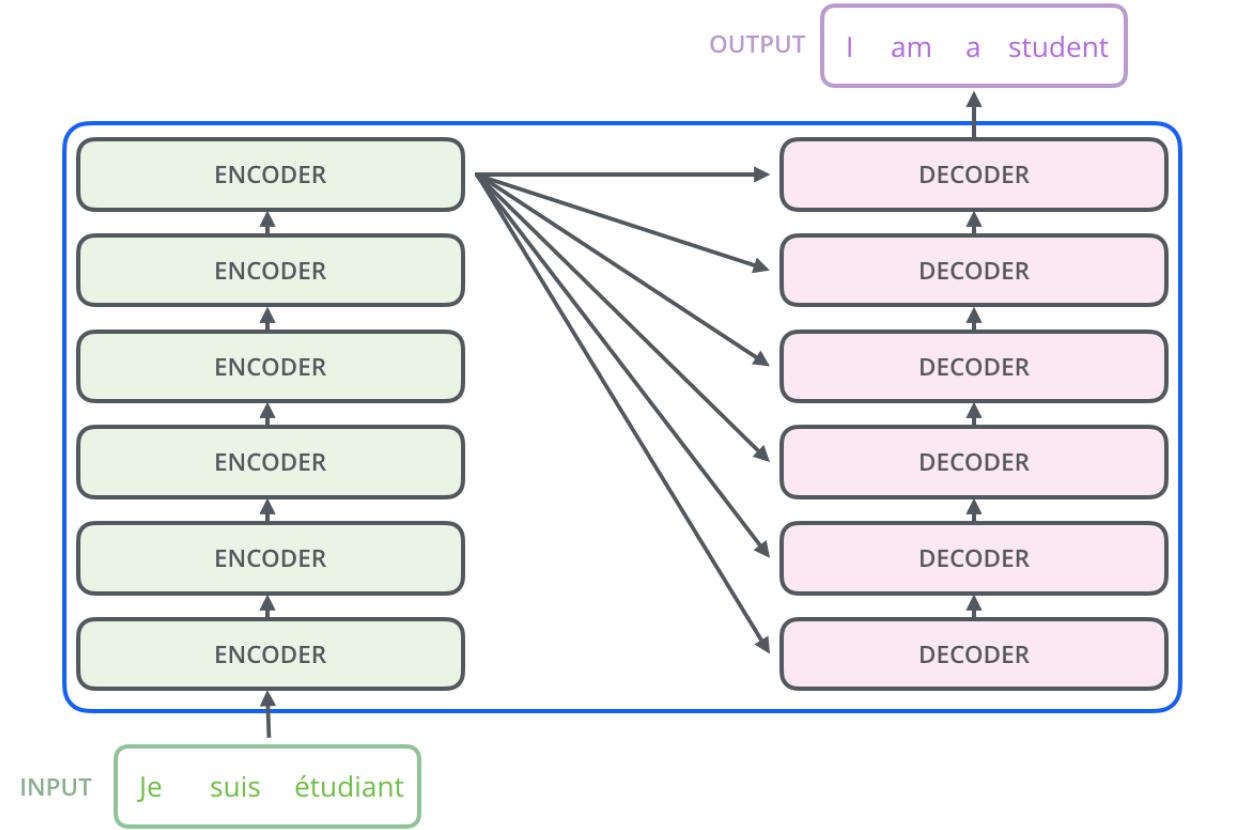
where \(\epsilon_t\) is white noise [2]. The encoder maps an input sequence \(\{x_1, \dots, x_n\}\) to representation sequence \(\mathbf{z} = \{z_1, \dots, z_n\}\). Then, the decoder generates an output sequence \(\{\hat{y}_1, \dots, \hat{y}_m\}\) from \(\mathbf{z}\) one element at a time.
- Notation
– \(\mathbf{q},\mathbf{k},\mathbf{v}\): query, key, and value row vectors
– \(Q,K,V\): matrices of \(\mathbf{q},\mathbf{k},\mathbf{v}\) respectively
– \(d_{model}\): the output dimension of all sub-layers and embedding layers, default=512
– \(d_{k}\): the dimension of keys and queries from the self-attention, default=64
– \(d_{v}\): the dimension of values from the self-attention, default=64
– \(d_{ff}\): the inner dimension of the feed-forward network, default=2048
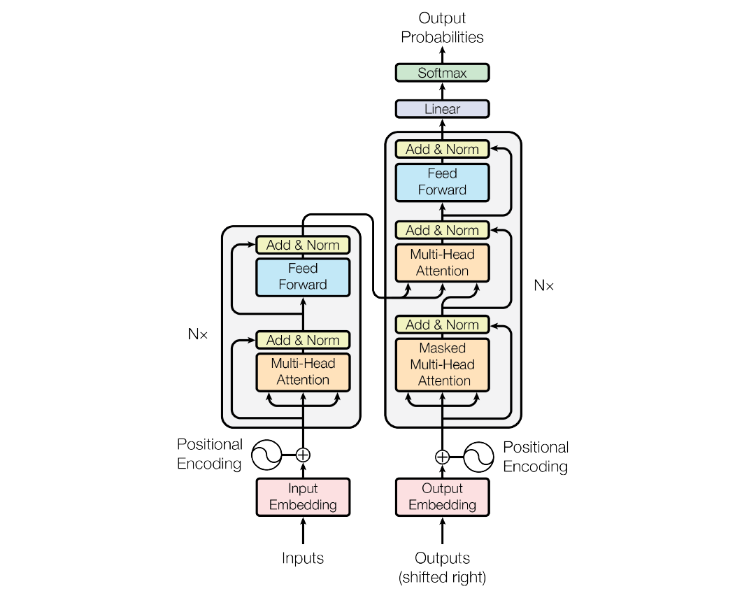
 figure 1: the transformer - model architecture.
1.1. Encoder and Decoder Stacks
Encoder
The encoder is composed of a stack of \(N\) identical NN blocks. Each block has 2 sub-layers: the first is a muti-head self-attention mechanism and the last is a fully connected feed-forward network. Both sub-layers employ residual connection followed by layer normalization.
Residual connection skips intermediate computations and adds the input directly to the output layer. This skip connection is known to assist error backpropagation.
Layer normalization is one of normalization techniques distinct to batch normalization. Batch normalization empirically estimates the mean and standard deviation of the entire data from mini-batch datasets. Due to the estimation method, however, the technique has constraints on the size of a mini-batch. Moreover, batch normalization is hard to apply to sequence data since the layer need to save some statistics for each time series order but sequences always have variable-length. On the other hand, layer normalization normalize representations in the same layer; i.e., it normalizes each sample at once. In addition, layer normalization performs equivalent computations in training and testing step since it uses identical gain and bias parameters for each time sequence unlike batch normalization [3].
Decoder
The decoder is same as the encoder except 2 properties. First, we need to make a word mask and feed it with input data into the decoder to prevent the self-attention sub-layer from peeking at the upcoming sequences. (Referring to the PyTorch tutorial, we also need to make the other masks to hide the padding tokens from both the encoder and decoder [4].) Second, another multi-head self-attention sub-layer is inserted between the masked multi-head attention layer and the feed-forward layer. The inserted layer takes a pair of keys and values from the encoder and queries from the masked multi-head attention layer.
 figure 2: encoder to decoder structure of the transformer. (source: http://www.aiotlab.org/teaching/intro2ai/slides/10_attention_n_bert.pdf)
1.2. Attention
An attention function takes queries and a pair of keys and values and print a weighted sum of the values. The weight are attained from a compatibility function of the query with the corresponding key.
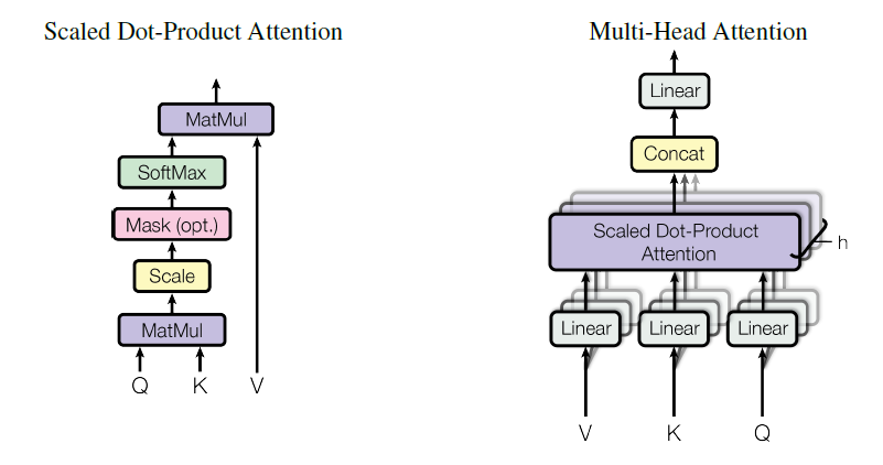
 figure 3: (left) scaled dot-product attention. (right) multi-head attention consists of several attention layers running in parallel.
1.2.1. Scaled Dot-Product Attention
The authors’ particular attention, scaled dot-product attention, calculates the dot products of the query with all keys, divides each by \(\sqrt{d_k}\), applies a softmax function to obtain the weights, and computes matrix multiplication between weights and values matrices. In practice, for the length \(n\) of a sequence, \[\begin{aligned} Attention(Q,K,V) &= softmax(\frac{QK^T}{\sqrt{d_k}})V \newline &= softmax(\frac{1}{\sqrt{d_k}} \begin{bmatrix} \mathbf{q}_1 \newline \vdots \newline \mathbf{q}_n \end{bmatrix} \begin{bmatrix} \mathbf{k}_1^T & \cdots & \mathbf{k}_n^T \end{bmatrix}) \begin{bmatrix} \mathbf{v}_1 \newline \vdots \newline \mathbf{v}_n \end{bmatrix} \newline &= \begin{bmatrix} softmax(\frac{1}{\sqrt{d_k}} \left[\mathbf{q}_1\mathbf{k}_1^T, \cdots, \mathbf{q}_1\mathbf{k}_n^T \right]) \newline \vdots \newline softmax(\frac{1}{\sqrt{d_k}} \left[\mathbf{q}_n\mathbf{k}_1^T, \cdots, \mathbf{q}_n\mathbf{k}_n^T \right]) \end{bmatrix} \begin{bmatrix} \mathbf{v}_1 \newline \vdots \newline \mathbf{v}_n \end{bmatrix} \newline &= \begin{bmatrix} p_{11} & \cdots & p_{1n} \newline \quad & \vdots & \quad \newline p_{n1} & \cdots & p_{nn} \end{bmatrix} \begin{bmatrix} \mathbf{v}_1 \newline \vdots \newline \mathbf{v}_n \end{bmatrix} \newline &= \begin{bmatrix} p_{11}\mathbf{v}_1 + \cdots + p_{1n}\mathbf{v}_n \newline \quad \vdots \quad \newline p_{n1}\mathbf{v}_1 + \cdots + p_{nn}\mathbf{v}_n \end{bmatrix}. \end{aligned}\]
For large \(d_k\), the dot products increase and then it causes the softmax function to have extreamly small gradients. Therefore the authors scale the dot product by \(\frac{1}{\sqrt{d_k}}\).
1.2.2. Multi-Head Attention
Instead of using a single attention directly, the model subjects queries, keys and values to \(h\) different trained linear transformations of the output dimensions \(d_k\), \(d_k\), and \(d_v\), respectively. Then the \(h\) outputs go through parallel attentions followed by concatenating and another linear projection. This multi-head attention structure makes the transformer possible to gain information jointly from different representation subspaces derived from \(h\) linear transformations. With a single attention head, averaging inhibits this. The entire procedure is expressed as follows: \[\begin{gathered} MultiHead(Q,K,V) = Concat(head_1, \dots, head_h)W^O \newline \text{where} \quad head_i = Attention(QW_i^Q,KW_i^K,VW_i^V) \newline \text{and} \quad W_i^Q \in \mathbb{R}^{d_{model} \times d_{k}}, W_i^K \in \mathbb{R}^{d_{model} \times d_{k}}, W_i^V \in \mathbb{R}^{d_{model} \times d_{v}}. \end{gathered}\]
1.2.3. Applications of Attention in the Model
The transformer uses muti-head attention in 3 different ways.
In enc2dec attention layers, the model takes queries from the previous layer in the same decoder block and keys and values from the terminal block of the encoder.
self-attention layers in the encoder takes all of the queries, keys and values from the previous encoder block. Each position(query) can attend to all positions(keys) in the previous block.
self-attention layers in the decoder similar to the decoder’s except that the softmax receives data with a mask of future positions to maintain the auto-regressive characteristic.
1.3. Position-wise Feed-Forward Networks
For each block in the encoder and decoder, every block has a fully connected feed-forward network followed by residual connection. The feed-forward sub-layer consists of 2 linear transformations with a ReLU activation in between. \[FFN(x) = \max(0, xW_1 + b_1)W_2 + b_2\]
The input and output dimensions are \(d_{model}\), and the inner dimension is \(d_{ff}\).
1.4. Embedding and Softmax
Similar to general seq2seq models, the transformer uses trained embeddings to take input and output tokens as vectors. The model also uses a learned linear transformation and softmax function to convert the decoder output to next-token probabilities. In addition, the embedding and the linear transformation shares the identical weight matrix. However, as we can see in the PyTorch tutorial, we can train the transformer and predict next-token, only except estimating probabilities, by argmax without weight tying and softmax function. Also we multiply the output by \(\sqrt{d_k}\) in the embedding layers.
1.5. Positional Encoding
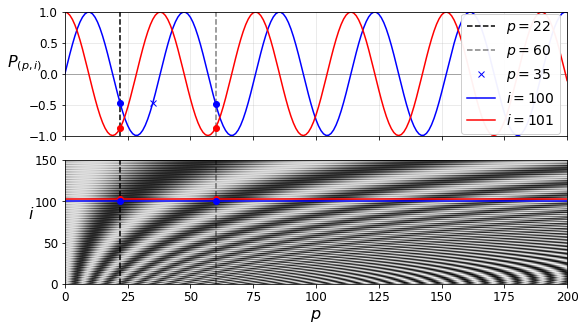
Since the transformer contains neither recurrence nor convolution, we have to prepare a way to transmit information about the absolute or relative position in the sequence in order for the model to make use of the order of the sequence. To this end, we make trainless “positional encodings” using sinusoidal function and add them to the output of the embeddings. For position \(pos\) and dimension \(i\) (\(0 \leq i \leq d_{model}-1\)), the positional encodings are: \[\begin{gathered} PE_{(pos, 2i)} = \sin(pos/10000^{2i/d_{model}}) \newline PE_{(pos, 2i+1)} = \cos(pos/10000^{2i/d_{model}}). \end{gathered}\]
Here, the bigger \(i\) is, the longer period is, resulting in a unique \(PE_{(pos)}\) for each \(pos\). This allows the model to figure out the absolute position of each token in the sequence. Besides, the model easily learns to attend by relative positions since \(PE_{pos}\) can be represented as a linear function of \(PE_{pos+k}\) for arbitrary fixed offset \(k\).

figure 4: sine and cosine positional encodings. (source: https://github.com/ageron/handson-ml2/blob/master/16_nlp_with_rnns_and_attention.ipynb)
Regularization
The authors use dropout and it is only applied to fully connected layers. In particular, the transformer apply dropout to the outputs of the multi-head attention and the feed-forward network respectively before normalized and the sums of the embeddings and the positional encodings [4, 5].
2. Why Self-Attention

Let us compare self-attention to recurrence and convolution in 3 aspects regarding the computation time for processing variable-length sequence. The 1st is the total computational complexity per layer. The 2nd is the amount of parallelizable computation, which is measured by the minimum number of sequential operations required. The 3rd is the length of the path to compute of long-range dependencies between tokens in the network. It is known that learning long-range dependencies is affected by the path length of forward and backward transmission. The shorter these paths, the easier it is to learn.
In terms of parallel computing, a self-attention layer connects all positions in a sequence with a constant number of operations, while recurrent layer requires \(O(n)\) sequential oprations.
With regard to the computational complexity, unrestricted self-attention has \(O(n^2 \cdot d)\) and we can find out that this runtime obtained from the number of multiplications in the computation in section 1.2.1. \(d > n\) is common in many cases of state-of-the-art transduction models.
Concerning convolution, a single convolutional layer with kernel width \(k < n\) cannot connect all positions. So it has \(O(n/k)\) or \(O(\log_k(n))\) maximum path length depending on its type. Also convolutional layers are generally expensive than recurrent layers in respect of computational complexity.
References
[1] Vaswani, Ashish, et al. “Attention is all you need.” Advances in neural information processing systems 30 (2017).
[2] Hyndman, R.J., & Athanasopoulos, G. (2021) Forecasting: principles and practice, 3rd edition, OTexts: Melbourne, Australia. OTexts.com/fpp3. Accessed on <2023-09-21>.
[3] Ba, Jimmy Lei, Jamie Ryan Kiros, and Geoffrey E. Hinton. “Layer normalization.” arXiv preprint arXiv:1607.06450 (2016).
[4] https://pytorch.org/tutorials/beginner/translation_transformer
[5] https://pytorch.org/docs/stable/_modules/torch/nn/modules/transformer
