Denoising Diffusion Probabilistic Models
review DDPM.
Generative deep learning models like VAEs and GANs have shown brilliant performance. “Denoising Diffusion Probabilistic Models” (DDPM) [1] is novel generative model published in 2020. This model is based on “Deep Unsupervised Learning Using Nonequilibrium Thermodynamics (2015)”.
1. What are diffusion probabilistic models?
 figure1: The directed graphical model considered in this work.
Diffusion probabilistic models (briefly, diffusion models) are latents variable models that handle latents of the same dimension as the original data. They are also parametrized Markov chains trained by variational inference to produce samples matching given data in finite time. Trainsitions in a chain (the probability of state change between events) are learned to reverse a diffusion process, which is a Markov chain that gradually add noise to the data in the opposite direction of sampling until signal is destroyed. If the diffusion process is a series of small amount of Gaussian noise, it is sufficient to set the sampling chain transitions to the posterior.
1.1. Diffusion and its reverse process
During the diffusion process \(q(\mathbf{x}_{1:T} \vert \mathbf{x}_0)\), for real data \(\mathbf{x}_0 \sim q(\mathbf{x}_0)\) and fixed small magnitude of variance schedule \(\{ \beta_t \in (0,1) \}^T_{t=1}\), the model gradually adds Gaussian noise to \(\mathbf{x}_0\), producing a sequence of noisy samples \(\mathbf{x}_1, \dots, \mathbf{x}_T\): \[q(\mathbf{x}_{1:T} \vert \mathbf{x}_0) = \underset{t=1}{\overset{T}{\prod}} q(\mathbf{x}_t \vert \mathbf{x}_{t-1}), \quad q(\mathbf{x}_t \vert \mathbf{x}_{t-1}) = \mathcal{N}(\mathbf{x}_t; \sqrt{1-\beta_t}\mathbf{x}_{t-1}, \beta_t\mathbf{I}) \qquad (1)\]
An impressive property of the diffusion process is that we can sample \(\mathbf{x}_t\) at an arbitrary timestep \(t\) in a closed form: Let \(\alpha_t = 1 - \beta_t\) and \(\bar{\alpha}_t = \prod^t_{s=1}\alpha_s\), then we have \[q(\mathbf{x}_t \vert \mathbf{x}_0) = \mathcal{N}(\mathbf{x}_t; \sqrt{\bar{\alpha}_t}\mathbf{x}_0, (1-\bar{\alpha}_t)\mathbf{I}) \qquad (2)\]
i.e., \(\mathbf{x}_t = \sqrt{\bar{\alpha}_t}\mathbf{x}_0 + \sqrt{(1-\bar{\alpha}_t)} \epsilon\) for \(\epsilon \sim \mathcal{N}(\mathbf{0}, \mathbf{I})\).
Meanwhile, during the reverse process \(p_{\theta}(\mathbf{x}_{0:T})\), we define it as a Markov chain with learned Gaussian transitions that approximate the posterior \(q(\mathbf{x}_{t-1} \vert \mathbf{x}_t)\) with \(p_{\theta}(\mathbf{x}_{t-1} \vert \mathbf{x}_t)\) starting at \(p(\mathbf{x}_t) = \mathcal{N}(\mathbf{x}_t;\mathbf{0},\mathbf{I})\): \[p_{\theta}(\mathbf{x}_{0:T})=p(\mathbf{x}_t)\underset{t=1}{\overset{T}{\prod}}p_{\theta}(\mathbf{x}_{t-1} \vert \mathbf{x}_t), \quad p_{\theta}(\mathbf{x}_{t-1} \vert \mathbf{x}_t) = \mathcal{N}(\mathbf{x}_{t-1}; \pmb{\mu}_{\theta}(\mathbf{x}_t,t), \mathbf{\Sigma}_{\theta}(\mathbf{x}_t,t)) \qquad (3)\]
Consequently, it models \(q(\mathbf{x}_0)\) as \(p_{\theta}(\mathbf{x}_0)=\int p_{\theta}(\mathbf{x}_{0:T})d_{\mathbf{x}_{1:T}}\).
To maximize the likelihood, we train a model by optimizing the variational bound on the negative log likelihood: \[\mathbb{E}[-\log p_{\theta}(\mathbf{x}_0)] \leq \mathbb{E}_q \left[-\log \frac{p_{\theta}(\mathbf{x}_{0:T})}{q(\mathbf{x}_{1:T} \vert \mathbf{x}_0)} \right] = \mathbb{E}_q \left[-\log p(\mathbf{x}_T) -\underset{t\geq1}{\sum}\log \frac{p_{\theta}(\mathbf{x}_{t-1} \vert \mathbf{x}_t)}{q(\mathbf{x}_t \vert \mathbf{x}_{t-1})} \right] =: L \qquad (4)\]
We can rewrite the loss for each \(t\) as: \[\mathbb{E}_q \left[D_{KL}(q(\mathbf{x}_T \vert \mathbf{x}_0) \parallel p(\mathbf{x}_T)) + \underset{t>1}{\sum}D_{KL}(q(\mathbf{x}_{t-1} \vert \mathbf{x}_t, \mathbf{x}_0) \parallel p_{\theta}(\mathbf{x}_{t-1} \vert \mathbf{x}_t)) -\log p_{\theta}(\mathbf{x}_0 \vert \mathbf{x}_1) \right] \qquad (5)\]
(For details, see appendix A of the paper.) It is noteworthy that the loss compares \(p_{\theta}(\mathbf{x}_{t-1} \vert \mathbf{x}_t)\) against \(q(\mathbf{x}_{t-1} \vert \mathbf{x}_t, \mathbf{x}_0)\) to approximate \(q(\mathbf{x}_{t-1} \vert \mathbf{x}_t)\), which is tractable when conditioned on \(\mathbf{x}_0\): \[\begin{gathered} q(\mathbf{x}_{t-1} \vert \mathbf{x}_t, \mathbf{x}_0) = \mathcal{N}(\mathbf{x}_{t-1}; \tilde{\pmb{\mu}}_t(\mathbf{x}_t, \mathbf{x}_0), \tilde{\beta}_t\mathbf{I}) \qquad (6) \newline \text{where} \quad \tilde{\pmb{\mu}}_t(\mathbf{x}_t, \mathbf{x}_0) = \frac{\sqrt{\bar{\alpha}_{t-1}}\beta_t}{1-\bar{\alpha}_t}\mathbf{x}_0 + \frac{\sqrt{\alpha_t}(1-\bar{\alpha}_{t-1})}{1-\bar{\alpha}_t}\mathbf{x}_t \quad \text{and} \quad \tilde{\beta}_t=\frac{1-\bar{\alpha}_{t-1}}{1-\bar{\alpha}_t}\beta_t \qquad (7) \end{gathered}\]
Let us label each component of the loss.
\(L_T = D_{KL}(q(\mathbf{x}_t \vert \mathbf{x}_0) \parallel p(\mathbf{x}_T))\)
\(L_{t-1} = D_{KL}(q(\mathbf{x}_{t-1} \vert \mathbf{x}_t, \mathbf{x}_0) \parallel p_{\theta}(\mathbf{x}_{t-1} \vert \mathbf{x}_t))\)
\(L_0 = -\log p_{\theta}(\mathbf{x}_0 \vert \mathbf{x}_1)\)
1.2. Parameterization of \(L_{T}\), \(L_{t-1}\) and \(L_{0}\)
\(L_{T}\)
\(p(\mathbf{x}_T) = \mathcal{N}(\mathbf{x}_t;\mathbf{0},\mathbf{I})\) is Gaussian noise and \(q(\mathbf{x}_t \vert \mathbf{x}_0)\) has no learnable parameters since DDPMs use fixed \(\beta_t\). These imply that \(L_{T}\) is constant and therefore it can be ignored.
\(L_{0}\)
To obtain discrete log likelihood, the authors set the last term of the reverse process as independent discrete decoder \(p_{\theta}(\mathbf{x}_0 \vert \mathbf{x}_1) \sim \mathcal{N}(\mathbf{x}_0; \pmb{\mu}_{\theta}(\mathbf{x}_1, 1), \sigma_1^2\mathbf{I})\). (\(\sigma_t\) is explained in the next paragraph.)
\(L_{t-1}\)
For \(1 < t \leq T\), we defined that \(p_{\theta}(\mathbf{x}_{t-1} \vert \mathbf{x}_t) = \mathcal{N}(\mathbf{x}_{t-1}; \pmb{\mu}_{\theta}(\mathbf{x}_t,t), \mathbf{\Sigma}_{\theta}(\mathbf{x}_t,t))\). The authors first set \(\mathbf{\Sigma}_{\theta}(\mathbf{x}_t,t) = \sigma_t^2\mathbf{I} \quad\) (where \(\quad \sigma_t^2=\beta_t \quad\) or \(\quad \sigma_t^2=\tilde{\beta}_t=\frac{1-\bar{\alpha}_{t-1}}{1-\bar{\alpha}_t}\beta_t.\) Refer to Python code S.3.2.) to untrained time dependent constants. Then to parameterize \(L_{t-1}\) with respect to \(\pmb{\mu}_{\theta}(\mathbf{x}_t,t)\), they used the following analysis: With \(p_{\theta}(\mathbf{x}_{t-1} \vert \mathbf{x}_t) = \mathcal{N}(\mathbf{x}_{t-1}; \pmb{\mu}_{\theta}(\mathbf{x}_t,t), \sigma_t^2\mathbf{I})\), \[L_{t-1} = \mathbb{E}_q \left[\frac{1}{2\sigma_t^2} \| \tilde{\pmb{\mu}}_t(\mathbf{x}_t, \mathbf{x}_0) - \pmb{\mu}_{\theta}(\mathbf{x}_t,t) \|^2 \right] + C \qquad (8)\]
where \(C\) is a constant that does not depend on \(\theta\). Through the parameterization, we see that \(\pmb{\mu}_{\theta}(\mathbf{x}_t,t)\) models \(\tilde{\pmb{\mu}}_t(\mathbf{x}_t, \mathbf{x}_0)\). Furthermore, by equations \((2)\)&\((7)\), we can express \(L_{t-1}\) as: \[L_{t-1} - C = \mathbb{E}_{\mathbf{x}_0, \pmb{\epsilon}} \left[\frac{1}{2\sigma_t^2} \| \frac{1}{\sqrt{\alpha_t}}(\mathbf{x}_t(\mathbf{x}_0, \pmb{\epsilon}) - \frac{\beta_t}{\sqrt{1-\bar{\alpha}_t}}\pmb{\epsilon}) - \pmb{\mu}_{\theta}(\mathbf{x}_t(\mathbf{x}_0, \pmb{\epsilon}), t) \|^2 \right] \qquad (9)\]
Therefore we need to make \(\pmb{\mu}_{\theta}\) predict \(\frac{1}{\sqrt{\alpha_t}}(\mathbf{x}_t - \frac{\beta_t}{\sqrt{1-\bar{\alpha}_t}}\pmb{\epsilon})\). Since \(\mathbf{x}_t\) is available in the model, we might choose the parameterization \[\pmb{\mu}_{\theta}(\mathbf{x}_t, t) = \frac{1}{\sqrt{\alpha_t}}(\mathbf{x}_t - \frac{\beta_t}{\sqrt{1-\bar{\alpha}_t}}\pmb{\epsilon}_{\theta}(\mathbf{x}_t, t)) \qquad (10)\]
where \(\pmb{\epsilon}_{\theta}\) is a function approximator to predict \(\pmb{\epsilon}\) from \(\mathbf{x}_t\). In the experiments, the authors’ own adapted U-net [2] is used as the function. From this \(\pmb{\mu}_{\theta}(\mathbf{x}_t, t)\), we can sample \(\mathbf{x}_{t-1} \sim p_{\theta}(\mathbf{x}_{t-1} \vert \mathbf{x}_t)\) by computing \(\mathbf{x}_{t-1} = \pmb{\mu}_{\theta}(\mathbf{x}_t, t) + \sigma_t\mathbf{z}\), where \(\mathbf{z} \sim \mathcal{N}(\mathbf{0},\mathbf{I})\).
By the parameterization of \(\pmb{\mu}_{\theta}\), \(L_{t-1}\) can be simplified to: \[\mathbb{E}_{\mathbf{x}_0, \pmb{\epsilon}} \left[\frac{\beta_t^2}{2\sigma_t^2\alpha_t(1-\bar{\alpha}_t)} \| \pmb{\epsilon} - \pmb{\epsilon}_{\theta}(\sqrt{\bar{\alpha}_t}\mathbf{x}_0 + \sqrt{1-\bar{\alpha}_t}\pmb{\epsilon}, t) \|^2 \right] \qquad (11)\]
The authors claim that empirically better results were yielded from the following unweighted loss function: \[L_{simple}(\theta) = \mathbb{E}_{t, \mathbf{x}_0, \pmb{\epsilon}} \left[ \| \pmb{\epsilon} - \pmb{\epsilon}_{\theta}(\sqrt{\bar{\alpha}_t}\mathbf{x}_0 + \sqrt{1-\bar{\alpha}_t}\pmb{\epsilon}, t) \|^2 \right] \qquad (12)\]
This corrsponds to \(L_{0}\) and \(L_{t-1}\) for the \(t\) = 1 case and the \(t\) > 1 cases respectively. (\(L_{T}\) is ignored since \(\beta_t\) are fixed.)
2. Python code
Let us talk about DDPM in TensorFlow, Python. The authors provide their code here. We will only look into the core file “diffusion-master/diffusion_tf/diffusion_utils.py” that contains theoretical contents. “diffusion_utils.py” is used in “diffusion-master/scripts/run_celebahq.py”.
Default setting:
Markov chain time steps \(T\) = 1000
\(\beta\) schedule = “linear” (linspace from 1e-4 to 2e-2)
2.1. Training
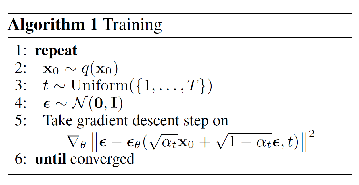
The following numberings do not correspond to each of pseudocodes.
T,S.0
Initialize the Model and load GaussianDiffusion in diffusion_utils.py. GaussianDiffusion contains almost all mathematical functions for the diffusion model.

Let’s follow the training code flow.
T.1
To train the Model, run Model.train_fn. For each input data in minibatch, sample \(t\) from uniform distrubution and use the constant \(t\). self._denoise load and return the adapted Unet. Now, let’s jump into GaussianDiffusion to look at self.diffusion.p_losses.
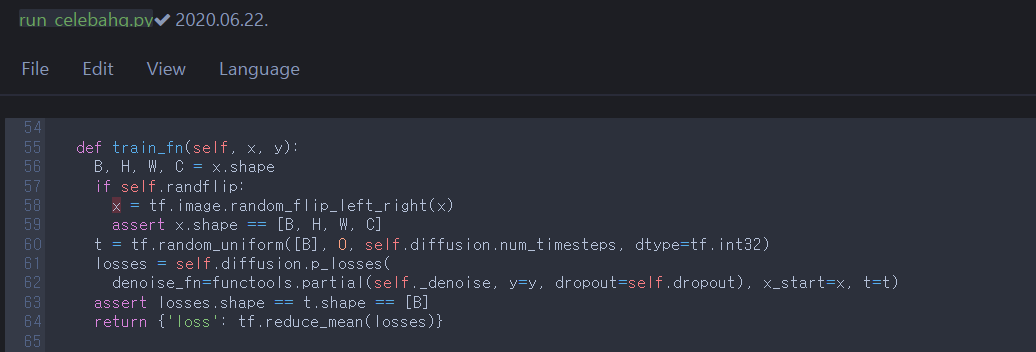
T.2
p_losses corresponds to the equation \((12)\), \(L_{simple}(\theta) = \mathbb{E}_{t, \mathbf{x}_0, \pmb{\epsilon}} \left[ \| \pmb{\epsilon} - \pmb{\epsilon}_{\theta}(\sqrt{\bar{\alpha}_t}\mathbf{x}_0 + \sqrt{1-\bar{\alpha}_t}\pmb{\epsilon}, t) \|^2 \right]\). As figured out in section 1.2, the parameterized and simplified variational bound minimizes difference between Gaussian noise \(\pmb{\epsilon}\) and model \(\pmb{\epsilon}_{\theta}\). self.q_sample is equivalent to sampling \(\mathbf{x}_t\) from \(q(\mathbf{x}_t \vert \mathbf{x}_0)\) (the equation \((2)\)) for an arbitrary \(t\). denoise_fn is the Unet and it estimates noise \(\pmb{\epsilon}_{\theta}\) from noisy sample \(\mathbf{x}_t\). nn.meanflat is just tf.reduce_mean with specific axis argument.
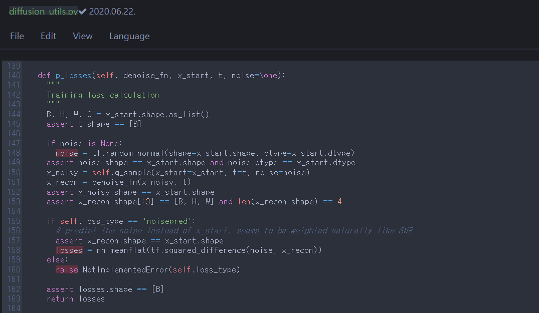
- The result: \(L_{simple}(\theta)\), returned from step 2.
2.2. Sampling
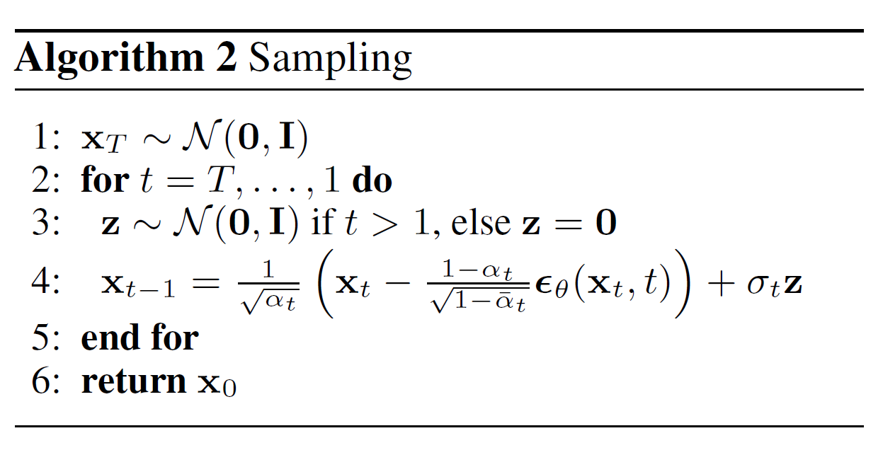
It’s time for the sampling code.
S.1
We need to run Model.samples_fn to generate samples. self.diffusion.p_sample_loop is a functions of GaussianDiffusion. It is the iteration of GaussianDiffusion.p_sample that samples \(\mathbf{x}_{t-1} \sim p_{\theta}(\mathbf{x}_{t-1} \vert \mathbf{x}_t)\) from \(T\) to \(1\); i.e., it returns synthetic sample \(\mathbf{x}_0\) from noise \(\mathbf{x}_T \sim \mathcal{N}(\mathbf{0},\mathbf{I})\). So, let’s take a look at p_sample.

S.2
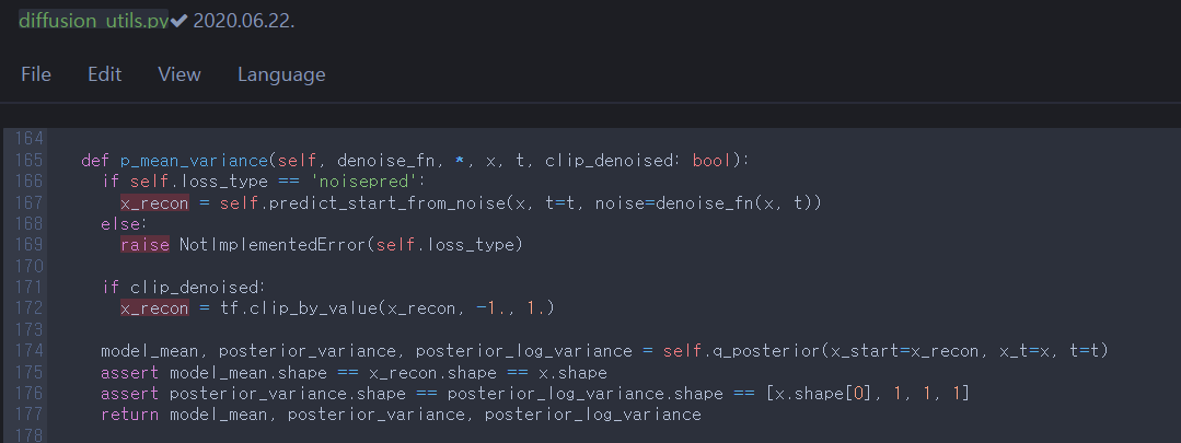
p_sample corresponds to \(\mathbf{x}_{t-1} \sim p_{\theta}(\mathbf{x}_{t-1} \vert \mathbf{x}_t)\) by computing \(\mathbf{x}_{t-1} = \pmb{\mu}_{\theta}(\mathbf{x}_t, t) + \sigma_t\mathbf{z} = \frac{1}{\sqrt{\alpha_t}}(\mathbf{x}_t - \frac{\beta_t}{\sqrt{1-\bar{\alpha}_t}}\pmb{\epsilon}_{\theta}(\mathbf{x}_t, t)) + \sigma_t\mathbf{z}\), where \(\mathbf{z} \sim \mathcal{N}(\mathbf{0},\mathbf{I})\). (It was mentioned between equations \((10)\)&\((11)\) in section 1.2). We need to compute p_mean_variance to obtain \(\pmb{\mu}_{\theta}(\mathbf{x}_t, t)\) and \(\log(\sigma_t^2)\).

S.3
There are predict_start_from_noise and q_posterior. Let’s take a look at each of them.
S.3.1
predict_start_from_noise is the reverse process of sampling \(\mathbf{x}_t\) from \(\mathbf{x}_0\) directly (q_sample, equation \((2)\)). So it returns \(\mathbf{x}_0\) from a noisy sample \(\mathbf{x}_t\), \(t\), and the estimated noise \(\pmb{\epsilon}_{\theta}\) between \(\mathbf{x}_t\)&\(\mathbf{x}_{0}\) by Unet.

S.3.2
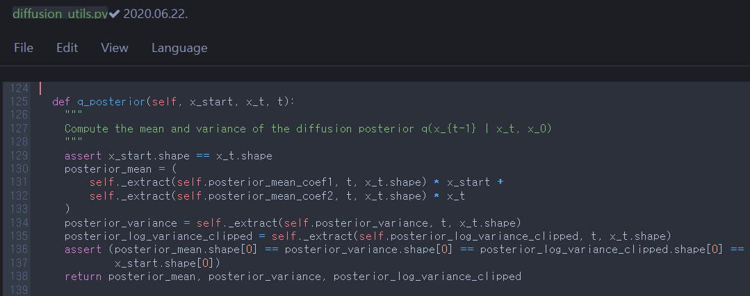
q_posterior is equivalent to equation \((7)\) and takes \(\mathbf{x}_{0}\), \(\mathbf{x}_{t}\), t. This \(\mathbf{x}_{0}\) came from predict_start_from_noise. It returns \(\tilde{\pmb{\mu}}_t(\mathbf{x}_t, \mathbf{x}_0)\), \(\sigma_t^2\) and \(\log{ \max (\text{1e-20}, \sigma_t^2)}\). Note that \(\sigma_t^2=\tilde{\beta}_t=\frac{1-\bar{\alpha}_{t-1}}{1-\bar{\alpha}_t}\beta_t\).
- The result: synthetic sample \(\mathbf{x}_0\), returned from step 1 as a result of the iteration.
Note
For many mathematical concepts and proofs, I recommend that you read lilianweng’s comprehensive posts 1 & 2.
Also it would be helpful to refer to the following review.
References
[1] Ho, Jonathan, Ajay Jain, and Pieter Abbeel. “Denoising diffusion probabilistic models.” Advances in neural information processing systems 33 (2020): 6840-6851.
[2] Ronneberger, Olaf, Philipp Fischer, and Thomas Brox. “U-net: Convolutional networks for biomedical image segmentation.” Medical Image Computing and Computer-Assisted Intervention–MICCAI 2015: 18th International Conference, Munich, Germany, October 5-9, 2015, Proceedings, Part III 18. Springer International Publishing, 2015.
