High-Resolution Image Synthesis With Latent Diffusion Models

27 Apr 2024 in Review

review Stable Diffusion.

In the image synthesis domain, diffusion models had shown very effective manipulation of images. However the models require abundant GPU calculations since they are operated in pixel space. To conserve computational resource while preserving flexibility and quality, Stable Diffusion (2022) [1] introduced latent space into the process.

Related review: Denoising Diffusion Probabilistic Models

1. Method

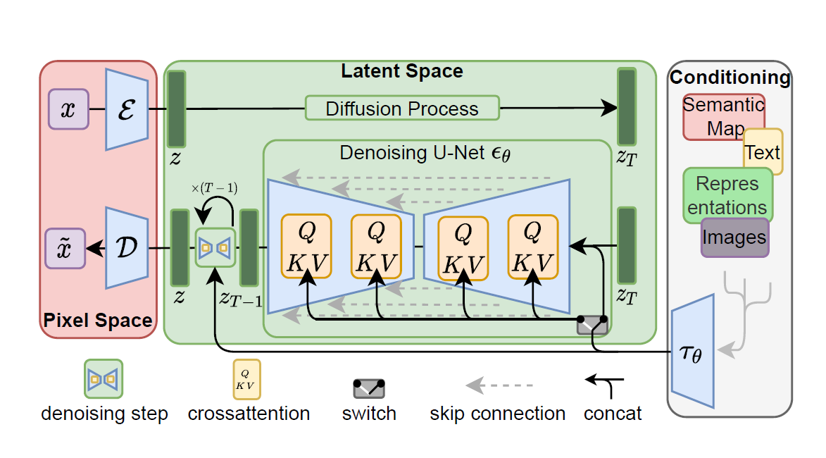figure1.1: Entire process of LDMs and its conditioning

Even though DDPM [2] ignores perceptually irrelevant details (especially estimating \(\epsilon\) instead of \(\tilde{\mu}\) and using the untrained time dependent constant \(\sigma_t^2\) instead of learning reverse process variance \(\sum_{\theta}(x_t)\)), calculation of the loss function in pixel space is still expensive. The authors detour such a shortcoming by explicitly seperating compression process and generative learning phase. To achieve this, they utilize an autoencoder model which learns latent space that not only has lower dimension number than the original space but also is perceptually equivalent. Such an approach has the following advantages:

1. It is efficient since sampling is processed in the latent space.
2. The diffusion model benefits by the inductive bias from UNet architecture which is effective to spartial structure, so it does not need to face the drawback from previous models [3, 4].
3. From the obtained latent space, it is available to do inpaint & text conditioning tasks or downsteam applications.

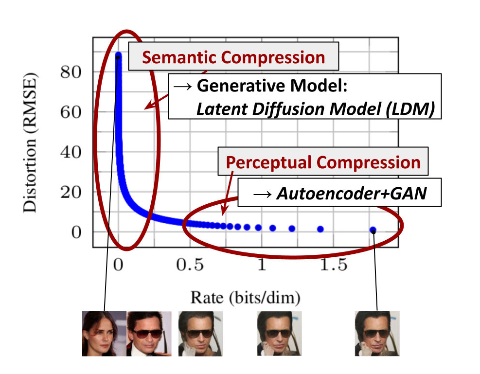figure1.2: Illustrating perceptual and semantic compression

1.1. Perceptual Image Compression

The autoencoder model used in Stable Diffusion is based on VQ-GAN [3] and trained by perceptual loss and patch-based adversarial objective. Also it is regulated by either KL-reg. or VQ-reg. loss term. The model using KL-reg. is similar to ordinary VAE [5, 6], while the other one uses a vector quantization layer [7] within the decoder.

The authors noted that “Interestingly, we find that LDMs trained in VQ-regularized latent spaces achieve better sample quality, even though the reconstruction capabilities of VQ-regularized first stage models slightly fall behind those of their continuous counterparts”.

1.2. Latent Diffusion Models

1.2.1. Diffusion Models

DDPM

The most successful diffusion models [2, 8, 9] learns real data distribution by gradually removing Gaussian distribution noise from data. Such denoising model learning is the reverse process of a fixed Markov chain with length \(T\). Also this denoising process can be interpreted as an equally weighted sequence of denoising encoders \(\epsilon_{\theta}(x_{t}, t)\) for \(t = 1,...,T\). To make a model has \[p_{\theta}(x_{t-1}|x_{t}) = \mathcal{N}(x_{t-1}; \mu_{\theta}(x_{t},t), \sigma_{t}^{2}I)\]

which approximates \[q(x_{t-1}|x_{t}, x_{0}) = \mathcal{N}(x_{t-1}; \tilde{\mu}_{t}(x_{t},x_{0}), \tilde{\beta}_{t}I),\]

for uniformly sampled \(t\), the models has the loss function: \[L_{DM} = \mathbb{E}_{x, \epsilon \sim \mathcal{N}(0,1), t}[\| \epsilon - \epsilon_{\theta}(x_{t},t) \|_2^2].\]

DDIM

The author of DDIM [10] generalized the Markovian diffusion process of DDPM to non-Markovian one (i.e., \(x_t\) depends on both \(x_{t-1}\) and \(x_0\).) while their model is still able to use the same loss function. They suggest that “Our key observation is that the DDPM objective in the form of \(L_{\gamma}\) only depends on the marginals \(q(x_t | x_0)\), but not directly on the joint \(q(x_{1:T} | x_0)\).”.

The benefits of DDIMs are:

1. We can accelerate denoising steps and generate higher quality sample by DDIMs based on their own method. i.e., DDIMs are faster than DDPMs.
2. For an initial latent variable and various steps, DDIMs consistently generate similar high-level features. (It is distingushed to the high diversicification of DDPM due to the stochastic generative process.)
3. This consistency enable users to interpolate images by manipulating the initial latent variable.

In brief, the reasons are:

• \(p_{\theta}(x_{t-1}|x_{t})\) of the generative process approximates \(q(x_{t-1}|x_{t}, x_{0})\) of the reverse process. For a real vector deviation \(\sigma \in \mathbb{R}_{\geq0}^T\) in diffusion process, suppose that \(\sigma \rightarrow 0 \quad \forall t\). Then \(q(x_{t}|x_{t-1}, x_{0})\) is deterministic (except \(t=1\)), and so \(p_{\theta}(x_{t-1}|x_{t})\) \(( \because x_{t-1} = \sqrt{\alpha_{t-1}} ( \frac{x_t - \sqrt{1-\alpha_t} \epsilon_{\theta}^{(t)}(x_t)}{\sqrt{\alpha_t}} ) + \sqrt{1-\alpha_{t-1} - \sigma_t^2} \cdot \epsilon_{\theta}^{(t)}(x_t) + \sigma_t \theta_t )\). It leads to that this model is an implicit probabilistic model. Based on these characteristics, the authors demonstrated the consistency in their experiments.

• On the other hand, since the loss function \(L_1\) does not depend on the specific diffusion procedure as long as \(q(x_{t}| x_{0})\) is fixed, we can consider a shorter subsequence process instead of original length \(T\) without another trained model. Thus the generative process is acceleratable. (For details, refer to Appendix C.1 in DDPM paper.)

Noise Schedule

Nichol et al (2021) [11] showed that the linear noise scheduler used in DDPM is too noisy, especially in the last quater of the diffusion process. For low resolution images such as \(64\times64\) or \(32\times32\), they demonstrated that the last 20% of diffusion process almost did not play a role in sample quality. Alternatively, they suggest a cosine scheduler, where \(\tilde{\alpha}_t\) is quasi-linear in the middle of the process and non-rapid near \(t=0\) and \(t=T\).

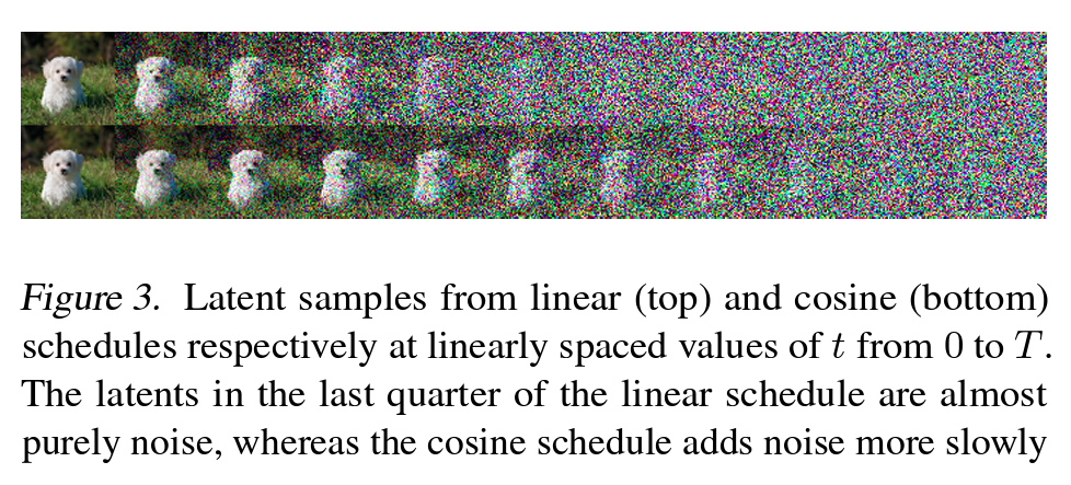figure1.3: Improved noise schedule

There are scheduler classes in latent-diffusion/ldm/lr_scheduler.py of the source code.

1.2.2. Generative Modeling of Latent Representations

Through VAE, we can access to perceptually compressive latent space. It is more adequate to likelihood-based generative models than pixel space because this latent space \((i)\) contains semantic bits, \((ii)\) is a low-dimensional efficient space. Since we are going to deal with latent code \(z_t = \mathcal{E}(x_t)\) for the encoder \(\mathcal{E}\), we update the loss function: \[L_{LDM} := \mathbb{E}_{\mathcal{E}(x), \epsilon \sim \mathcal{N}(0,1), t}[\| \epsilon - \epsilon_{\theta}(z_{t},t) \|_2^2].\]

The backbone model \(\epsilon_{\theta}\) is a time-conditional UNet [12].

1.3. Conditioning Mechanisms

Similar to other type of generative models [13, 14], DMs are capable of modeling conditional distribution of the form \(p(z|y)\). This can be implemented with a conditional denoising autoencoder \(\mathcal{E}_\theta(z_{t},t,y)\) and diversified to txt2img, semantic maps or other img2img tasks. Such features are realized by applying cross-attention mechanism into UNet backbone. To deal with \(y\) from various modalities, \(y\) is projected to a representation \(\tau_{\theta}(y) \in \mathbb{R}^{M \times d_r}\) through domain specific encoder \(\tau_{\theta}\). Then this \(\tau_{\theta}(y)\) is mapped to the intermediate layers of UNet via a cross-attention layer. The attention operation is: \[\begin{gathered} Attention(Q,K,V) = softmax(\frac{QK^T}{\sqrt{d}}) \cdot V, \newline \text{with} \quad Q = W_Q^{(i)} \cdot \varphi_i(z_t), K = W_K^{(i)} \cdot \tau_{\theta}(y), V = W_V^{(i)} \cdot \tau_{\theta}(y). \end{gathered}\]

Here, \(\varphi_i(z_t) \in \mathbb{R}^{N \times d_{\epsilon}^{i}}\) denote a flatten intermediate representation of the UNet \(\mathcal{E}_\theta\) and \(W_Q^{(i)} \in \mathbb{R}^{d \times d_{\epsilon}^{i}}, W_K^{(i)} \in \mathbb{R}^{d \times d_r}, W_V^{(i)} \in \mathbb{R}^{d \times d_r}\) are learnable projection matrices. From these, the updated loss function is: \[L_{LDM} := \mathbb{E}_{\mathcal{E}(x), y, \epsilon \sim \mathcal{N}(0,1), t}[\| \epsilon - \epsilon_{\theta}(z_{t},t,\tau_{\theta}(y)) \|_2^2]\]

where \(\tau_{\theta}\) & \(\epsilon_{\theta}\) are pairwise optimized.

2. Python Code

Open source code of Stable Diffusion

model config: txt2img-1p4B-eval.yaml for text2img task

Let’s figure out the essential code part.

2.1. main.py

Train or test depending on opt.

figure2.1.1 <== 2,3,4,8

parser opt

figure2.1.2

Trainer is pytorch_lightning.trainer.Trainer

figure2.1.3 <== 7

model

instantiate_from_config is in latent-diffusion/ldm/util.py and loads modules by referring to the config.

figure2.1.4 <== 5

config

figure2.1.5 <== 6

opt.base

figure2.1.6 <== 7

parser argument logdir

From 5, 6 and 7, we can find out that user needs to fill “logs/configs/” directory with yaml to start training initially when logdir is set as default to “logs”.

figure2.1.7

data

figure2.1.8

2.2. ldm/util.py

instantiate_from_config

In case of config.model[“target”] = ldm.models.diffusion.ddpm.LatentDiffusion, the result is LatentDiffusion(the dictionary of “params”) where “params” is in config.

figure2.2.1

2.3. ldm/models/diffusion/ddpm.py

LatentDiffusion.__init__(dict)

DDPM takes in unet_config.

first_stage_config is a config for VAE. In this case, it is AutoencoderKL, not VQModel.

cond_stage_config is a config for a domain specific encoder. In this case, it is BERTEmbedder for text conditioning.

figure2.3.1

Load a VAE and a domain specific encoder.

figure2.3.2

p_losses function with conditional argument for Stable Diffusion

figure2.3.3

log_images function handles input & condition, plots, samples, and returns log dictionary. we focus on the sampling.

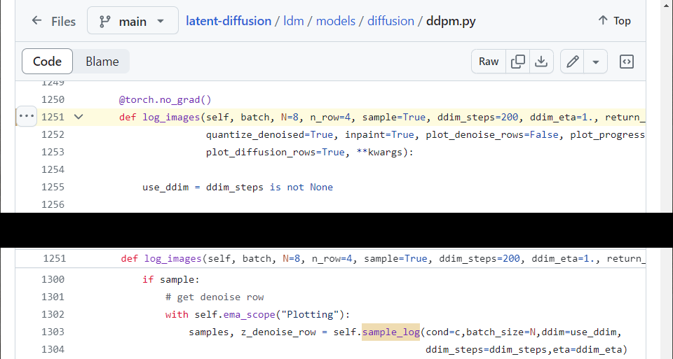figure2.3.4

Here, either DDIM or DDPM sampling method is chosen.

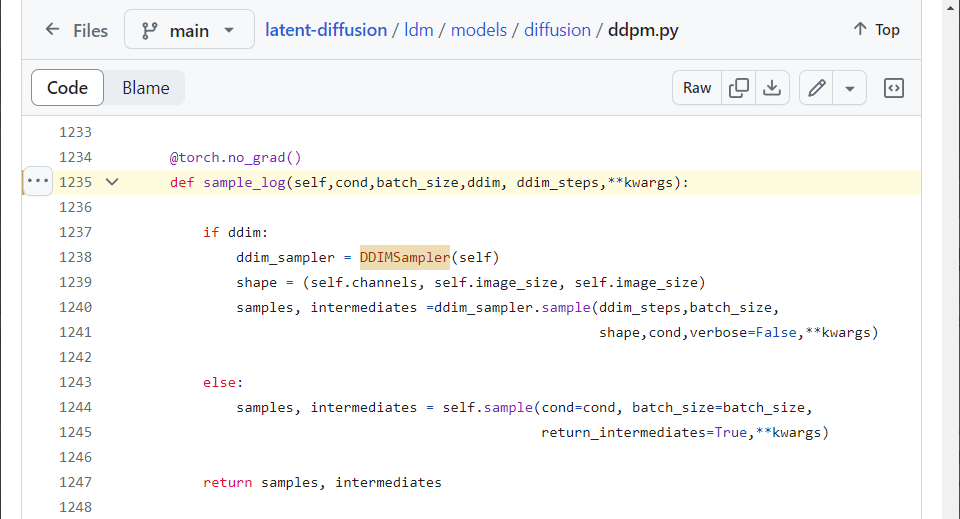figure2.3.5

2.4. ldm/modules/attention.py

CrossAttention \(\rightarrow\) BasicTransformerBlock \(\rightarrow\) SpatialTransformer

This is \(Attention(Q,K,V) = softmax(\frac{QK^T}{\sqrt{d}}) \cdot V\) where \(Q, K, V\) are linear projections of \(\varphi_i(z_t), \tau_{\theta}(y), \tau_{\theta}(y)\) respectively.

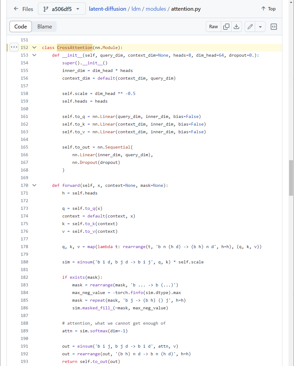figure2.4.1

This is a simple Transformer block similar to the one of GPT-2.

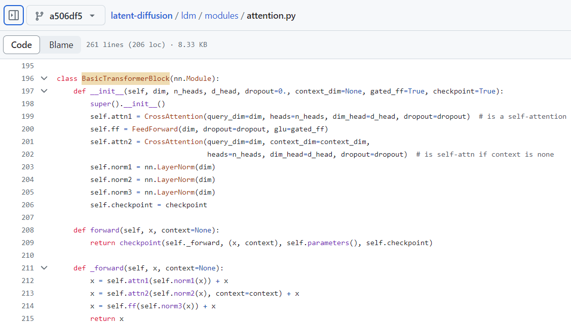figure2.4.2

SpatialTransformer deals with image-like data using the Transformer based architecture. The input is projected by Conv2d and rearranged before processed. (Note that inner_dim = heads * dim_head (the number of attention heads and the dimension of each head), default: heads=8, dim_head=64.)

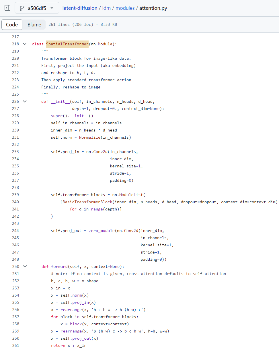figure2.4.3

2.5. ldm/modules/encoders/modules.py

These are pretrained BERTTokenizer and the corresponding BERTEmbedder \(= \tau_{\theta}\).

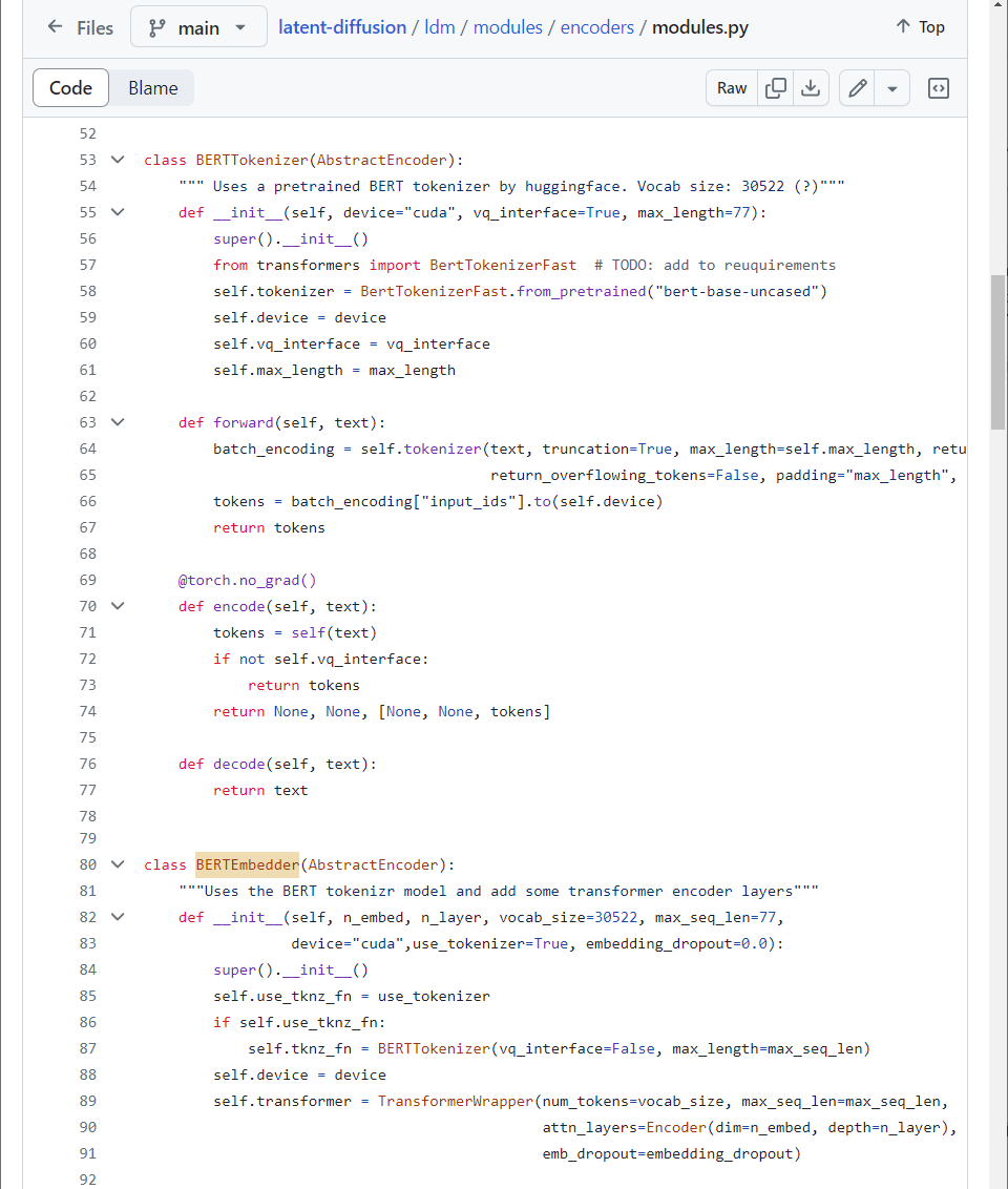figure2.5.1

2.6. ldm/modules/losses/contperceptual.py

These are the loss terms and the training procedure for the continuous VAE based on VQ-GAN.

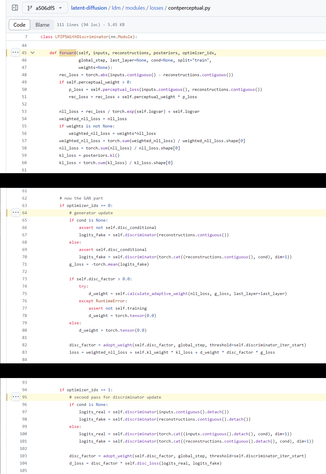figure2.6.1

2.7. scripts/txt2img.py

Finally, sample images from a trained model. Default initial latent code \(x_T\) is a Gaussian noise. model.ema_scope is of Exponential Moving Average.

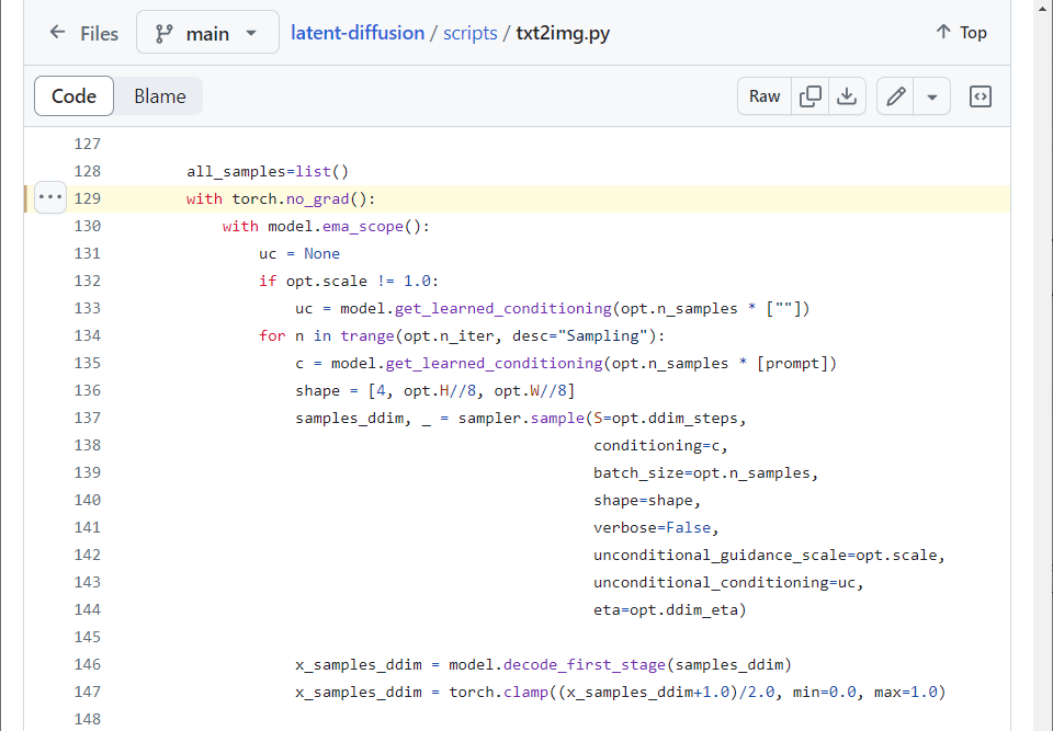figure2.7.1

References

[1] Rombach, Robin, et al. “High-resolution image synthesis with latent diffusion models.” Proceedings of the IEEE/CVF conference on computer vision and pattern recognition. 2022.

[2] Ho, Jonathan, Ajay Jain, and Pieter Abbeel. “Denoising diffusion probabilistic models.” Advances in neural information processing systems 33 (2020): 6840-6851.

[3] Esser, Patrick, Robin Rombach, and Bjorn Ommer. “Taming transformers for high-resolution image synthesis.” Proceedings of the IEEE/CVF conference on computer vision and pattern recognition. 2021.

[4] Ramesh, Aditya, et al. “Zero-shot text-to-image generation.” International conference on machine learning. Pmlr, 2021.

[5] Diederik P. Kingma and MaxWelling. Auto-Encoding Variational Bayes. In 2nd International Conference on Learning Representations, ICLR, 2014. 1, 3, 4, 27

[6] Danilo Jimenez Rezende, Shakir Mohamed, and Daan Wierstra. Stochastic backpropagation and approximate inference in deep generative models. In Proceedings of the 31st International Conference on International Conference on Machine Learning, ICML, 2014. 1, 4, 27

[7] Van Den Oord, Aaron, and Oriol Vinyals. “Neural discrete representation learning.” Advances in neural information processing systems 30 (2017).

[8] Prafulla Dhariwal and Alex Nichol. Diffusion models beat gans on image synthesis. CoRR, abs/2105.05233, 2021. 1, 2, 3, 4, 6, 7, 8, 15, 19, 23, 24, 26

[9] Chitwan Saharia, Jonathan Ho, William Chan, Tim Salimans, David J. Fleet, and Mohammad Norouzi. Image super-resolution via iterative refinement. CoRR, abs/2104.07636, 2021. 1, 4, 7, 19, 20, 21, 25

[10] Jiaming Song, Chenlin Meng, and Stefano Ermon. Denoising diffusion implicit models. In ICLR. OpenReview.net, 2021. 3, 5, 6, 20

[11] Nichol, Alexander Quinn, and Prafulla Dhariwal. “Improved denoising diffusion probabilistic models.” International conference on machine learning. PMLR, 2021.

[12] Ronneberger, Olaf, Philipp Fischer, and Thomas Brox. “U-net: Convolutional networks for biomedical image segmentation.” Medical Image Computing and Computer-Assisted Intervention–MICCAI 2015: 18th International Conference, Munich, Germany, October 5-9, 2015, Proceedings, Part III 18. Springer International Publishing, 2015.

[13] Mehdi Mirza and Simon Osindero. Conditional generative adversarial nets. CoRR, abs/1411.1784, 2014. 4

[14] Kihyuk Sohn, Honglak Lee, and Xinchen Yan. Learning structured output representation using deep conditional generative models. In C. Cortes, N. Lawrence, D. Lee, M. Sugiyama, and R. Garnett, editors, Advances in Neural Information Processing Systems, volume 28. Curran Associates, Inc., 2015. 4